Show code cell source Hide code cell source

# stdlib
from pathlib import Path
import matplotlib.pyplot as plt
import numpy as np

# wcomp
from wcomp import WCompFloris, WCompPyWake, WCompFoxes
from wcomp.plotting import plot_plane

# plot settings
PROFILE_LINEWIDTH = 1.0
ERROR_LINEWIDTH = 1.5

SMALL_SIZE = 10
MEDIUM_SIZE = 12
BIGGER_SIZE = 14
# plt.rc('font', size=SMALL_SIZE)          # controls default text sizes
plt.rc('xtick', labelsize=SMALL_SIZE)    # fontsize of the tick labels
plt.rc('ytick', labelsize=SMALL_SIZE)    # fontsize of the tick labels
plt.rc('axes', labelsize=MEDIUM_SIZE)
plt.rc('axes', titlesize=BIGGER_SIZE)
plt.rc('legend', fontsize=MEDIUM_SIZE)
plt.rc('figure', titlesize=BIGGER_SIZE)

# Constants for all cases. Copy to a particular code block to change, as needed.
CASE_DIR = Path('cases_torque2024/one_turbine')
this_case = CASE_DIR / Path('jensen/wind_energy_system.yaml')
floris_case = WCompFloris(this_case)
ROTOR_D = floris_case.rotor_diameter
XMIN = -1 * ROTOR_D
XMAX = 20 * ROTOR_D
YMIN = -2 * ROTOR_D
YMAX =  2 * ROTOR_D

Dashboard

This page contains a series of cases that compare various aspects of the integrated wake modeling software including the mathematical wake models and other software-specific design decisions.

Wake model implementations

The mathematical models included in each software are generally grouped into models describing the velocity of the wind in a wind turbine wake (velocity model) and models describing the magnitude of deflection of the wake (deflection model). The models available in each software are shown in the tables below.

Table 1 Velocity models

Wake Model	FLORIS	FOXES	PyWake
Jensen 1983	•	•	•
Larsen 2009			•
Bastankhah / Porte Agel 2014		•	•
Bastankhah / Porte Agel 2016	•	•
Niayifar / Porté-Agel 2016			•
IEA Task 37 Bastankhah 2018			•
Carbajo Fuertes / Markfort / Porté-Agel 2018			•
Blondel / Cathelain 2020			•
Zong / Porté-Agel 2020			•
Cumulative Curl 2022	•
TurbOPark (Nygaard 2022)	•	•	•
Empirical Gauss 2023	•

Table 2 Deflection models

Wake Model	FLORIS	FOXES	PyWake
Jimenez 2010	•		•
Bastankhah / Porte Agel 2016	•	•
Larsen et al 2020			•
Empirical Gauss 2023	•

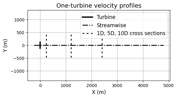
1-dimension wake profiles

Show code cell source Hide code cell source

x_turbine = np.array([0.0, 0.0])
y_turbine = np.array([-ROTOR_D/2, ROTOR_D/2])
x_streamwise = np.array([XMIN, XMAX])
y_streamwise = np.array([0.0, 0.0])
x_1d = np.array([1 * ROTOR_D, 1 * ROTOR_D])
x_5d = np.array([5 * ROTOR_D, 5 * ROTOR_D])
x_10d = np.array([10 * ROTOR_D, 10 * ROTOR_D])
y_crosswise = np.array([YMIN, YMAX])

fig, ax = plt.subplots(figsize=(6, 3))
ax.plot(x_turbine, y_turbine, '-', color='black', linewidth=3, label="Turbine")
ax.plot(x_streamwise, y_streamwise, '-.', color='black', linewidth=2, label="Streamwise")
ax.plot(x_1d, y_crosswise, linestyle=(0, (2, 3)), color='black', linewidth=2)
ax.plot(x_5d, y_crosswise, linestyle=(0, (2, 3)), color='black', linewidth=2)
ax.plot(x_10d, y_crosswise, linestyle=(0, (2, 3)), color='black', linewidth=2, label="1D, 5D, 10D cross sections")
ax.set_title("One-turbine velocity profiles")
ax.set_xlabel("X (m)")
ax.set_ylabel("Y (m)")
ax.set_ylim([-1000, 1000])
ax.axis('equal')
ax.grid()
ax.legend()

<matplotlib.legend.Legend at 0x7f7698b05af0>

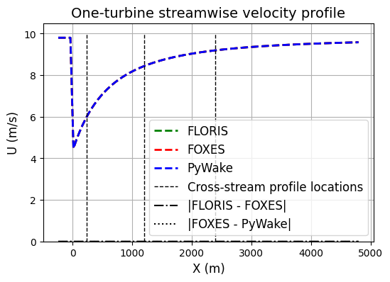
Jensen

Show code cell source Hide code cell source

this_case = CASE_DIR / Path('jensen/wind_energy_system.yaml')
floris_case = WCompFloris(this_case)
foxes_case = WCompFoxes(this_case)
pywake_case = WCompPyWake(this_case)

fig, ax = plt.subplots(figsize=(6,4))
floris_case.streamwise_profile_plot(wind_direction=270, y_coordinate=0.0, xmin=XMIN, xmax=XMAX)
foxes_case.streamwise_profile_plot(wind_direction=270, y_coordinate=0.0, xmin=XMIN, xmax=XMAX)
pywake_case.streamwise_profile_plot(wind_direction=270, y_coordinate=0.0, xmin=XMIN, xmax=XMAX)
ax.plot([1*ROTOR_D, 1*ROTOR_D], [0, 10], color="black", linestyle='--', linewidth=PROFILE_LINEWIDTH)
ax.plot([5*ROTOR_D, 5*ROTOR_D], [0, 10], color="black", linestyle='--', linewidth=PROFILE_LINEWIDTH)
ax.plot([10*ROTOR_D, 10*ROTOR_D], [0, 10], color="black", linestyle='--', linewidth=PROFILE_LINEWIDTH, label="Cross-stream profile locations")
lines = ax.lines
x1, y1 = lines[0].get_data()
x2, y2 = lines[1].get_data()
x3, y3 = lines[2].get_data()
e1 = np.abs(y1 - y2)
e2 = np.abs(y2 - y3)
ax.plot(x1, e1, color="black", linestyle='-.', linewidth=ERROR_LINEWIDTH, label="|FLORIS - FOXES|")
ax.plot(x1, e2, color="black", linestyle=':', linewidth=ERROR_LINEWIDTH, label="|FOXES - PyWake|")
ax.set_title("One-turbine streamwise velocity profile")
ax.set_xlabel("X (m)")
ax.set_ylabel('U (m/s)')
ax.set_ybound(lower=0.0)
ax.legend()
ax.grid()

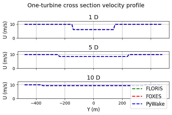
fig, ax = plt.subplots(3, 1, figsize=(6,4))
fig.suptitle("One-turbine cross section velocity profile")
X_D = [1, 5, 10]
for i, D_X in enumerate(X_D):
    plt.axes(ax[i])
    floris_case.xsection_profile_plot(wind_direction=270, x_coordinate=D_X * ROTOR_D, ymin=YMIN, ymax=YMAX)
    foxes_case.xsection_profile_plot(wind_direction=270, x_coordinate=D_X * ROTOR_D, ymin=YMIN, ymax=YMAX)
    pywake_case.xsection_profile_plot(wind_direction=270, x_coordinate=D_X * ROTOR_D, ymin=YMIN, ymax=YMAX)
    ax[i].set_title(f"{D_X} D")
    ax[i].set_ylabel("U (m/s)")
    ax[i].set_ybound(lower=0.0, upper=12.0)
    ax[i].grid()
    if i < len(X_D) - 1:
        ax[i].xaxis.set_ticklabels([])
    else:
        ax[i].set_xlabel("Y (m)")
        ax[i].legend()
fig.tight_layout()

Turbine 0, T0: windio_turbine

Grid points

Dropdown content

Rotor velocity average

Dropdown content

Partial wake

Dropdown content

Spatial discretization and rotor average velocity

Since the focus is specifically on analytical wake models, this class of software does not require a specific type of grid to model the wake. In practice, each software can choose a grid that meets its design and use objectives. However, the grid type has an impact on the results of the model through the computation of the thrust coefficient from a rotor-averaged velocity. The grid-types and methods for rotor averaging are compared here.

Point placement

Show the locations in space and note that the points are used in combination with a velocity average method.

Rotor velocity average

Develop a test case that demonstrates how the rotor-averaged velocity method performs. Ideally, this would be case that compares the methods outside the context of a wake model simulation, so something like average a function that analytically averages to 1.

Partial wake treatment

Describe how the rotor average velocity is computed for a turbine where part of the rotor is waked.

Grid dependency

plot of some quantity that's a function of the incoming wind (power, rotor average velocity...) as a function of grid resolution

Overlapping wakes

The mathematical models included in each software are generally grouped into models describing the velocity of the wind in a wind turbine wake (velocity model) and models describing the magnitude of deflection of the wake (deflection model). The models available in each software are shown in the tables below.

Wind shear and veer

Compare how the software model wind shear and wind veer

Software projects described

gantt dateFormat YYYY-MM-DD axisFormat %Y todayMarker off section FLORIS 0.1 :2018-01-16, 2019-05-07 1.0 :2019-05-07, 2020-04-27 2.0 :2020-04-27, 2020-06-23 2.1 :2020-06-23, 2020-09-25 2.2 :2020-09-25, 2021-05-01 2.3 :2021-05-01, 2021-10-02 2.4 :2021-10-02, 2022-02-25 2.5 :2022-02-25, 2022-03-01 3.0 :2022-03-01, 2022-04-06 3.1 :2022-04-06, 2022-09-16 3.2 :2022-09-16, 2023-03-07 3.3 :2023-03-07, 2023-05-16 3.4 :2023-05-16, 2023-10-26 3.5 :2023-10-26, 2024-03-15 3.6 :2024-04-05, 2024-04-09 4.0 :2024-04-09, 2024-06-01 section FOXES 0.1 (alpha) :2022-07-01, 2022-10-22 0.2 (alpha) :2022-10-22, 2023-01-27 0.3 (alpha) :2023-01-27, 2023-06-12 0.4 :2023-06-12, 2023-12-13 0.5 :2023-12-13, 2024-02-12 0.6 :2024-02-12, 2024-05-08 0.7 :2024-05-08, 2024-06-01 section PyWake 0.1 :2018-12-03, 2019-01-10 1.0 :2019-01-10, 2020-04-14 1.1 :2020-04-14, 2020-04-17 2.0 :2020-04-17, 2020-09-15 2.1 :2020-09-15, 2021-03-26 2.2 :2021-03-26, 2022-03-18 2.3 :2022-03-18, 2022-07-06 2.4 :2022-07-06, 2023-02-15 2.5 :2023-02-15, 2024-06-01

Fig. 1 Timeline of software releases